Nowadays time-series data are ubiquitous, from mobile networks, IoT devices to finance markets. Moving average is a simple yet fundamental method when it comes to time-series data analysis. For example, MA crossover is one of the strategies applied to quantitative trading. Here we can find how to compute moving average using Python, SQL and R.
The Data
We retrieve the daily stock market data for Google and Apple from Yahoo via pandas-datareader between 01/01/2012 to 30/06/2019. Then save the data into one DataFrame.
1
2
3
4
5
6
7
8
9
10
11
12
13
def retrieve_data(start_dt, end_dt, symbol_list):
    """Collect the stock market data"""
    df = pd.DataFrame()
    for s in symbol_list:
        tmp_df = pdr.DataReader(s, 'yahoo', start_dt, end_dt)
        tmp_df['Symbol'] = s
        if df.empty:
            df = tmp_df
        else:
            df = df.append(tmp_df)

    df.to_csv('./data/stocks.csv')
    return df
Compute moving average using Pandas
Pandas come with rich sets of functions for time-series / financial data analysis. I think that is because Wes McKinney, Pandas creator, is coming from financial background. We can simply apply the DataFrame function rolling followed by mean function. We will get the moving avereage of the given window. There are more parameters we can specify if we want to have different types of rolling window, i.e. exponential. In addition to this, we need to use groupby function in order to calculate the moving average for each symbol.
1
2
3
4
5
6
7
def compute_ma(df, window):
    """Compute the moving average of Adj Close for each Symbol"""
    ma_name = 'ma{0:d}'.format(window)
    df[ma_name] = (df.groupby('Symbol', sort=False)['Adj Close']
                    .rolling(window).mean()
                    .reset_index(0, drop=True))
    return df
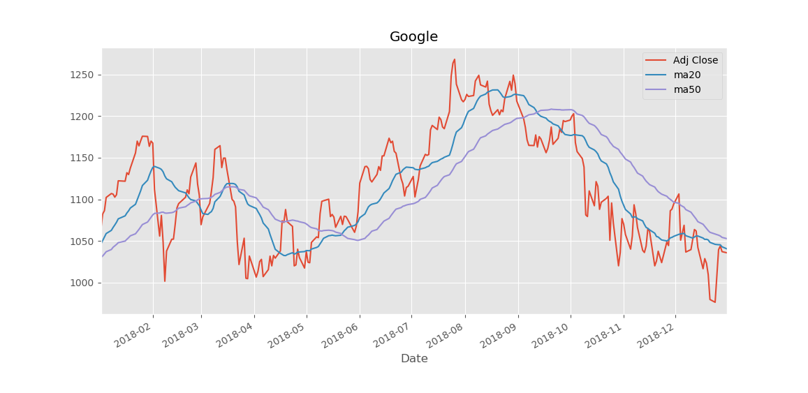
Pandas also makes it very handy to plot the time-series data. It is recommended to set the timestamp as index. So you just need to specify which columns and conditions you want to show. Pandas will handle the x-axis as proper Date type in the background.
1
2
df[(df['Symbol']=='GOOG') & (df.index.year==2018)][['Adj Close', 'ma20', 'ma50']].plot(title='Google')
plt.show()
Compute moving average with SQL (BigQuery)
We can use window functions in SQL to calculate the moving average for each symbol. If we want to get the results based on date range, the trick is the window_frame_clause is only supported numeric expression in BigQuery. We need to convert Date into integer with UNIX_DATE funtion before applying the window function. Here is the SQL statement in BigQuery.
1
2
3
4
5
6
7
8
9
10
11
12
13
SELECT
  Date,
  Symbol,
  Adj_Close,
  AVG(Adj_Close) OVER (
    PARTITION BY Symbol ORDER BY UNIX_DATE(Date) ASC
    RANGE BETWEEN 19 PRECEDING AND CURRENT ROW
    ) AS ma20,
  AVG(Adj_Close) OVER (
    PARTITION BY Symbol ORDER BY UNIX_DATE(Date) ASC
    RANGE BETWEEN 49 PRECEDING AND CURRENT ROW
    ) AS ma50
FROM my_dataset.stocks
If we just want to compute the moving average from the preceding N records to current record, we can use ROWS instead of RANGE. The SQL statement looks like below.
1
2
3
4
5
6
7
8
9
10
11
12
13
SELECT
  Date,
  Symbol,
  Adj_Close,
  AVG(Adj_Close) OVER (
    PARTITION BY Symbol ORDER BY Date ASC
    ROWS BETWEEN 19 PRECEDING AND CURRENT ROW
    ) AS ma20,
  AVG(Adj_Close) OVER (
    PARTITION BY Symbol ORDER BY Date ASC
    ROWS BETWEEN 49 PRECEDING AND CURRENT ROW
    ) AS ma50
FROM my_dataset.stocks
Compute moving average with data.table in R
data.table provides fast rolling functions to calculate aggregation on sliding windows, such as frollmean, froolsum. So it is basically one line of code to compute the moving average for a given window thanks to the flexible syntax of data.table.
1
2
3
4
5
6
7
8
9
10
11
12
library(data.table)
library(lubridate)

compute_ma <- function(dt, window) {
  dt <- dt[, paste0("ma", window) := lapply(.SD, frollmean, n=window, fill=NA),
           by=c("Symbol"), .SDcols=c("Adj Close")]
}

dt <- fread("./data/stocks.csv")
dt$Date <- ymd(dt$Date)
dt <- compute_ma(dt, 20)
dt <- compute_ma(dt, 50)